Recent architecture used in superconducting qubit processors
Coupling Types
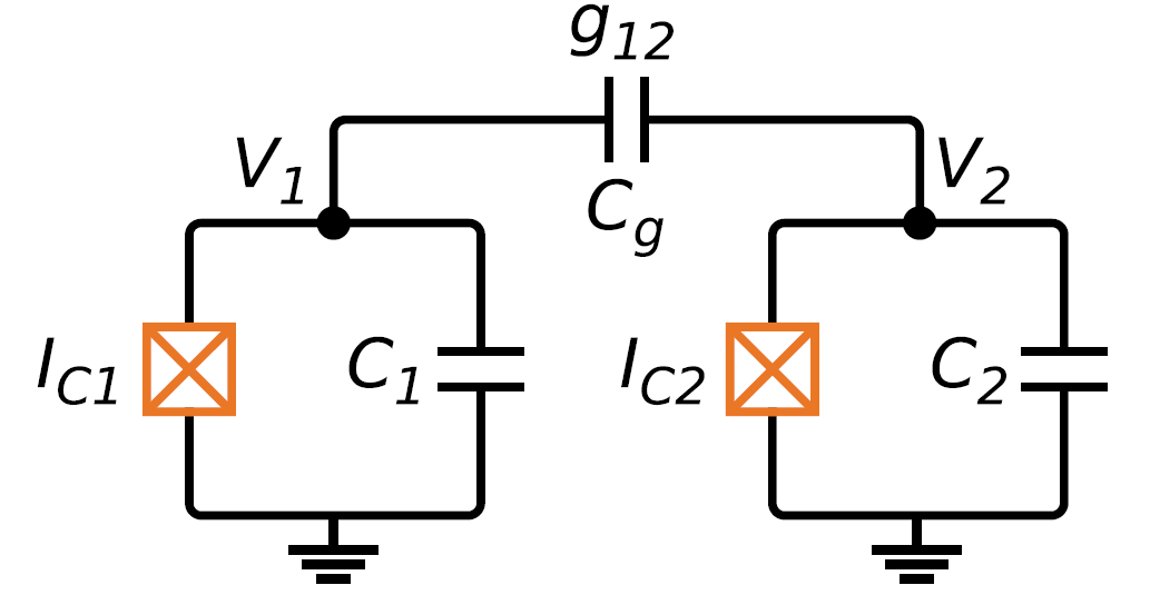
Fixed capacitive coupling
Each transmon qubit is coupled through a fixed capacitance creating the coupling strength \(g_{12}\) as shown in Fig. 1.
\begin{equation} \hat{H}/\hbar = \sum_{i=1,2}\left({\omega_{q,i} \hat{b}_i^\dagger \hat{b}_i + \frac{\alpha_{q,i}}{2} \hat{b}_i^\dagger \hat{b}_i^\dagger \hat{b}_i \hat{b}_i} \right)+ g_{12} \left( \hat{b}_1^\dagger + \hat{b}_1 \right)\left( \hat{b}_2^\dagger + \hat{b}_2 \right) \end{equation}
The Hamiltonian of the system is given in Eq. (1), where the coupling strength is given by \(g_{12} = \frac{2E_{C1}E_{C2}}{E_c} \left( \frac{E_{J1}}{2E_{C1}} \times \frac{E_{J2}}{2E_{C2}} \right)^{1/4}\) [1].
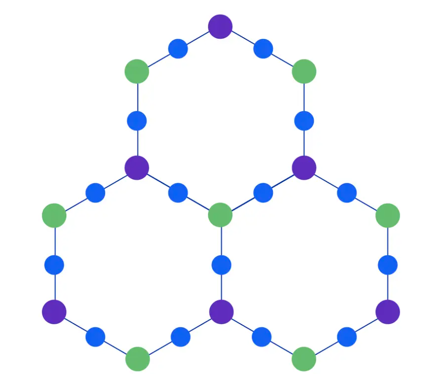
This coupling scheme inspires the heavy hexagonal architecture adapted by IBM Quantum in its early processors such as IBM Condor and its predecessors, illustrated in Fig. 2 [3, 4]. However, more connectivity among the qubits increases the vulnerability to frequency collisions.
Tunable coupler based
Each transmon qubit is coupled through a tunable transmon coupler with higher frequency maintaining the dispersive interaction.
\begin{equation} \hat{H}/\hbar = \sum_{i=1,2}\left({\omega_{q,i} \hat{b}_i^\dagger \hat{b}_i + \frac{\alpha_{q,i}}{2} \hat{b}_i^\dagger \hat{b}_i^\dagger \hat{b}_i \hat{b}_i} \right)+ \sum_{i\neq j} g_{ij} \left( \hat{b}_i^\dagger + \hat{b}_i \right)\left( \hat{b}_j^\dagger + \hat{b}_j \right) \end{equation}
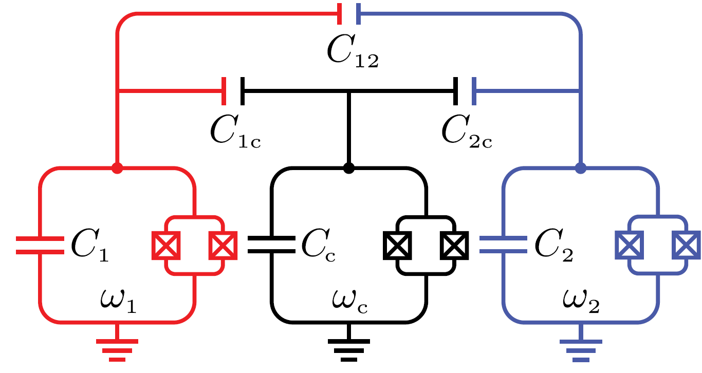
The Hamiltonian is as shown in Eq. (2), where each coupling strengths can be expressed in terms of the coupling capacitances: \(g_1 \approx \frac{1}{2} \frac{C_{1c}}{\sqrt{C_1 C_c}} \sqrt{\omega_1 \omega_c}\), \(g_2 \approx \frac{1}{2} \frac{C_{2c}}{\sqrt{C_2 C_c}} \sqrt{\omega_2 \omega_c}\), and \(g_{12} \approx \frac{1}{2} \left[ \frac{C_{12}}{\sqrt{C_1 C_2}} + \frac{C_{1c}C_{2c}}{\sqrt{C_1 C_2 C_c^2}} \right] \sqrt{\omega_1 \omega_2}\) [].
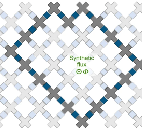
Recently, this scheme gains popularity due to the potential of isolating some qubits with the tunable coupling strength. This scheme inspires the square lattice used by Google Quantum AI [6], along with some processors developed by ETH Zurich [7], USTC [8], and IQM Finland [9]. IBM Quantum has also started to adopt this scheme, beginning from IBM Heron [10].
References
[1] A Blais et al, Circuit quantum electrodynamics, Reviews of Modern Physics 93, 025003 (2021)
[2] P Krantz et al, A quantum engineer’s guide to superconducting qubits, Applied Physics Reviews 6, 021318 (2019)
[3] https://research.ibm.com/blog/heavy-hex-lattice
[4] C Chamberland et al, Topological and Subsystem Codes on Low-Degree Graphs with Flag Qubits, Phys. Rev. X 10, 011022 (2020)
[5] F Yan et al, Tunable Coupling Scheme for Implementing High-Fidelity Two-Qubit Gates, Physical Review Applied 10, 054062 (2018)
[6] Google Quantum AI, Suppressing quantum errors by scaling a surface code logical qubit, Nature 614, pages 676–681 (2023)
[7] F Swiadek et al, Enhancing dispersive readout of superconducting qubits through dynamic control of the dispersive shift: Experiment and theory, PRX Quantum 2024
[8] Y Wu et al, Strong quantum computational advantage using a superconducting quantum processor, Physical Review Letters 127 (18), 180501
[9] https://aws.amazon.com/cn/blogs/quantum-computing/amazon-braket-launches-new-54-qubit-superconducting-quantum-processor-from-iqm/
[10] https://www.ibm.com/quantum/blog/large-scale-ftqc
Enjoy Reading This Article?
Here are some more articles you might like to read next: